Runtime Intent Drift: What an AI Workload Actually Does

Why AI agents fail without actually “failing”?

A conventional application failure is easier to detect and diagnose. It either panics, returns 500s, or a dashboard turns red.

An agent’s bad day looks like a normal day. It opens a file, runs a command, makes an outbound connection. Every operation is permitted and unremarkable in isolation. The problem is that this file, this command and this destination are not things this workload has ever needed.

Take a documentation-sync agent for example. Its regular job is to read markdown, summarize it through a model API, and write to a PostgreSQL database. One afternoon it reads a credentials directory and connects to a host it has never contacted. No authorization check fails, because the service account has filesystem read and general egress. There is no apparent crash and the audits don’t show any discrepancies in particular.

Two questions follow. How do you decide whether what a workload just did is behaviorally consistent? And how do you find out whether your answer is any good? We’ll discuss both with more focus on the second part.

“What can it do?” vs “What does it do?”

Service names, manifests, IAM policies and tool declarations ( AGENTS.md or SKILL.md file ) all state what a thing is supposed to do. We can call it the declared purpose of the agent. They describe intent at provisioning time. When they eventually go stale, they provide little value in describing an agent’s behavior at runtime.

AWS documents the gap directly. It recommends starting from managed policies, warns those “might not grant least-privilege permissions for your specific use cases because they’re available for use by all AWS customers”. The usual playbook here is to wait a sample period, review what was actually accessed, then write a replacement policy. As a result, granted permissions begin broader than exercised permissions by design, and the documented approach is to examine what the workload actually did, then rightsize.

So runtime intent here means something narrow: the behavior a workload has consistently demonstrated. Not its declared purpose, and not an inference about its business function. We cannot infer a workload’s true intent and are not trying to.
Declared purpose has its uses and is discussed later along with its architectural consequences.

Workload baselining

tenant + cluster + namespace + workload name

Key design choice we decided on is the granularity of capture. We do capture behavioral metrics at the pod, and process level. But both change on every restart and deploy, so a pod-scoped baseline spends its life relearning and never accumulates enough history to be useful. So for this purpose we stick to a workload level ( can be Deployment, DaemonSet and so on ).

Cluster belongs in the key because the same workload name behaves differently across environments. Staging hits test endpoints at a fraction of the volume and gets poked by engineers at odd hours. What counts as ordinary traffic in staging, rarely translates to more periodic production traffic.

Proposed design. The evaluation prototype described later keys baselines without a tenant dimension. Tenant isolation is separate.

Nine behavior families

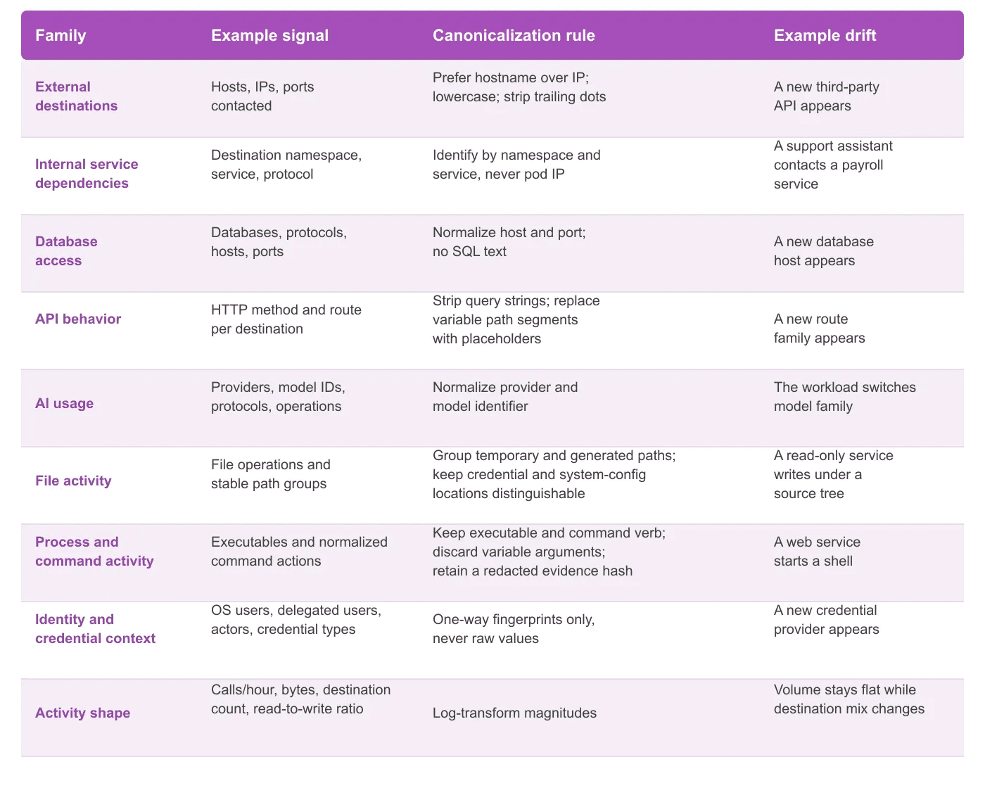
Two properties need special attention.

The family names are a contract. What lives inside a family will change, while the names will not. This helps maintain compatibility across versions while giving flexibility to change the scoring mechanism later on.

Canonicalization as a precondition. Route normalization is an example of this:

/customers/10291/orders/7
/customers/88420/orders/9
->  /customers/:id/orders/:id

Without that collapse, every ordinary customer ID is a value the workload has never seen, and the API family produces permanent, meaningless drift. The same applies to preferring hostnames over IPs, which rotate without any behavior change behind them, and to command arguments, which must not become baseline keys.

One choice we made for simplicity: We only describe database connection patterns and volume, not complete SQL text ( even though we do capture them ). The first version makes no claim about detecting changes in what queries mean. It would require another level of normalization that we can tackle later.

Handling missing telemetry

If file capture is not enabled on a cluster, “no file activity” is reported for that sensor. This is important to reduce the number of false positives reported because of operational reasons like misconfiguration.

So families become ready independently, and coverage gets reported:

External destinations: ready
File activity:         learning
AI usage:              ready
Process activity:      incomplete
Overall:               6 of 9 families ready

The proposed rules for baselining: a categorical family needs 7 complete days, at least 20 relevant events, spread across at least three distinct hours. Activity shape needs 24 non-empty hourly periods. A family that hits its distinct-value ceiling is marked incomplete and stops producing novelty findings ( as it would be very noisy ). The distinct value ceiling is configurable for each family type and can be done in retrospect.

Seven days is a bootstrap setting, which is too little to model weekly or seasonal patterns. We are not claiming it is sufficient in general, but is a good default to begin with. Separately, when new telemetry is switched on, that family starts its own learning period.

Proposed design. The evaluation prototype implements no readiness concept ( assumed ready ).

The maths behind it all

Each family ( or axis ) has its own way of evaluating:

Categorical signals are not numeric. Standard deviation does not apply to a set of hostnames or command name. Three separate questions matter here for set-like fields: has this value ever been seen, how often did it appear during learning, and how much has the mix of values shifted. The third question is important here. A workload moving from 95% service A to 95% service B introduces no new value but has plainly changed what it does. Jensen-Shannon divergence gives that a bounded number.

Numeric signals are often bursty rather than bell-shaped. A single nightly batch job drags the mean and inflates the spread until nothing looks anomalous. The proposal is median, median absolute deviation, and observed p95 and p99, applied to log(1 + value).

Combination is for cases where independence assumptions fail. A plain noisy-OR combines per-signal scores as 1 - Π(1 - wᵢnᵢ) and assumes independence. Ours are not independent. Small example to showcase this:
A workload has near 50-50 traffic split to external domain A and external domain B. But 90% of its traffic to A is read-only while 90% of its traffic to B is write. Simply considering external-endpoint and activity-type independently won’t raise a drift for cases where workload writes to A or reads from B.
So we collapse correlated families first, then combine:

Reach     = max(external, internal, database, API)
Execution = max(file, process)
AI usage  = ai
Identity  = identity
Activity  = activity shape

raw   = 1 - product(1 - group_score)
final = min(raw, strongest_group_score + 0.15)

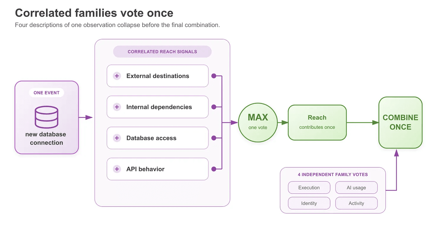
The cap keeps the property that makes noisy OR useful. The one serious change is enough on its own, while denying four descriptions of the same event the ability to compound.

How to test a drift detector?

Everything above is design. This section describes a prototype we built and ran.

The method:

Baseline hygiene decides whether any of it means anything. If an injected unit leaks into training, the baseline learns the drift and then fails to flag it, and recall collapses for reasons unrelated to the scorer being tested.

The corpus is generated to establish ground truth. Production traffic rarely has complete ground-truth labels ( at least at the start ), so you cannot compute recall against it, because you do not know what you missed.

Difficulty tiers, because a single accuracy number hides everything interesting. T1 is a value far outside the baseline, the sanity floor. T2 is a rare but previously seen value. T3 is recombination, accumulation and off-cadence activity, where every individual value is known and only the combination is new. T3 separates methods, and it resembles a careful adversary.

The five configurations ( approaches ):

Each model configuration receives a structured, redacted run summary together with the workload’s behavioral baseline. The volume-evidence configuration uses a different prompt variant from the other gated one, and the gated and unconditional configurations use different model sizes. They are five complete configurations, each differing in more than one respect, and not a controlled experiment isolating the gate.

Per-run calibration for noise removal

A naive categorical score uses 1 - P(value) from the baseline frequency table. But on a skewed axis, this flags almost every clean run. A forty-event run will usually contain at least one rare value, so finding an “unusual” value is normal.

Pooled frequency and per-run share measure different things. Pooled frequency tells us how common a value is across the workload’s history. Per-run share tells us whether that value occupies more or less of the current run than usual. Per-run here can be considered as an agentic session.

A host might generate a third of the workload’s total traffic while still varying widely between runs. Scoring against its pooled frequency mistakes that normal variation for a deviation. Scoring against observed run-to-run variation, while accounting for the extra noise in shorter runs, avoids this problem.

What we measured

The evaluation below comes from a locally reproduced corpus: six synthetic workloads over 30 days at generator seed 7, split 70/30 temporally, giving 576 training and 287 evaluation units per run; injection budget 0.15 across difficulty tiers T1 0.30, T2 0.35, T3 0.35; four injection seeds (42 through 45); per-run scoring granularity; run 4 August 2026. Counts below are pooled across the four seeds.

The co-occurrence result

A single-axis scorer cannot express a tuple. It examines commands and it examines hosts, but has no representation for “this command has never contacted this host”. Both values are individually ordinary, so nothing fires.

Adding a co-occurrence axis changed which categories of drift were detectable, rather than merely improving a score.

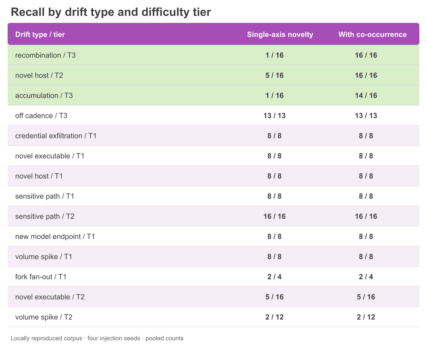
Co-occurrence recovered the cases it was designed to represent: recombination rose from 1 of 16 to 16 of 16, novel-host T2 from 5 of 16 to 16 of 16, and accumulation from 1 of 16 to 14 of 16. Most T1 categories were caught at 8 of 8, but fork fan-out reached only 2 of 4 for both configurations, so the sanity control did not pass universally. Both configurations also performed poorly on novel executable and volume spike at T2.

Across four seeds, single-axis F1 ranged from 0.592 to 0.658, while co-occurrence ranged from 0.765 to 0.833. The full observed ranges were 0.066 and 0.068 respectively.

Beyond the counting scorer

Everything above detects structural drift: a new host, command, path or credential pairing. Counting catches that cheaply and explains itself afterwards, which matters when a human has to adjudicate.

Semantic drift is different. A workload uses only sanctioned hosts, commands and paths, and pursues a non-specific goal. It produces no structural anomaly, because structurally nothing is wrong.

A model placed behind the behavioral gate does not solve this. The gate does not open on activity that is statistically insignificant, so semantic drift never reaches the adjudicator and the model that might recognize it is never asked.

The proposed response is that “declared scope” has to be machine-checkable, so a purpose baseline can participate in the gate decision rather than only in the prompt. The gate then opens on behavioral surprise or on out-of-scope access. As a production source for “declared scope” we are proposing to derive it from each agent’s manifest (AGENTS.md or SKILL.md), and make it part of the gate evaluation itself.

No evaluation so far has contained a valid intent-drift cell. A purpose-aware configuration produced verdicts identical to the behavior-only one, which reflects the absence of the case the purpose baseline exists to catch rather than a finding about declared purpose. A possible way of doing this is to reduce the threshold of the structural gate to allow more datapoints to flow to the LLM decider. But this would come at a cost of precision ( with improved recall ). Wiring them into the run path and adding scope definitions to the generated corpus is the next evaluation step, not a blocker requiring production workloads.

Three prototype limits remain. Cold start is unhandled: a workload with no history has no baseline and produces no verdict. There is no incremental update or decay, since baseline construction is a full batch recompute over the training window. Also, user feedback loop is something to be considered for manual baseline recompute. Slow accumulation is a known limitation of this prototype’s independent per-run scoring, which evaluates each run without reference to the ones before it.

Operating this without teaching it the wrong thing

Proposed design decisions, most of which exist to prevent one outcome: a detector that quietly learns an attacker’s activity as normal.

Baseline versions are immutable. An active baseline never changes in place; any change creates a new version linked to its parent. That buys an audit trail of what counted as normal at any past moment, reproducible scores, and rollback without rebuilding from raw events.

New categorical behavior is never learned automatically. A reviewer marks a signal as an expected change and explicitly approves a successor baseline containing it, and every approval records who, when, and which signal justified it. Marking something a false positive informs threshold calibration without specifically allow-listing the record.

The proposed rollout begins in shadow mode, recording candidate drift for review with no customer-visible threat and no notification. Deduplication is keyed on workload, baseline version, dominant family, changed-feature fingerprint and calendar week, so a persistent change updates one record instead of alerting hourly.

One deliberate omission: the first version detects newly introduced and unusually large behavior, not the disappearance of expected behavior. Missing calls are usually idleness, scaling or an outage, and telling those apart from a silenced agent needs a different model.

Key Takeaways